Introduction
This post summarizes ongoing research on optimal execution under endogenous MEV. The goal is to move beyond treating MEV as a static surcharge and instead model it as an equilibrium outcome: execution costs depend on how adversaries infer and respond to your execution policy.
Decentralized exchanges now route very large volumes through public, algorithmic market structures. That transparency enables a family of adversarial strategies—front-running, back-running, and sandwiching—that are collectively described as Maximal Extractable Value (MEV). In many practical settings, execution policies are highly structured (e.g., TWAP-style schedules), which makes intent partially inferable and invites strategic response.
Classical optimal execution (e.g., Almgren–Chriss) assumes that market impact is an exogenous friction: the control problem trades off impact against risk. In DeFi, that assumption is often violated. Impact and MEV losses are policy-dependent because the adversary’s behavior is endogenous.
We formalize this interaction as a Stackelberg game between a large trader (leader) and a best-responding searcher population (followers). We then approximate equilibrium policies using Iterated Best Response (IBR) and use the resulting framework to identify a complexity frontier: the conditions under which adaptive policies (including recurrent RL with guardrails) provide measurable benefits over simple execution heuristics such as TWAP.
Model: The Execution Game
The Stackelberg Formulation
We formalize the interaction as a sequential game:
- Leader (Trader): Commits to an execution policy $\pi_T$ (a distribution over schedules). Commitment here is behavioral: the follower observes realized execution signals (recent blocks, timing/size patterns) and best-responds.
- Follower (Searcher): Observes the policy and chooses an extraction strategy (attack decision + sizing rule) to maximize profit. We assume the follower conditions on recent execution history and current pool state.
The trader's objective is to minimize total cost (Implementation Shortfall + MEV losses): $$ J_T(\pi_T) = \mathbb{E}\left[\text{IS} + \sum_{t=1}^T \text{MEV}_t(\pi_T, \text{BR}(\pi_T))\right] $$ where $\text{BR}(\pi_T)$ is the searcher's best response.
Automated Market Maker (AMM) Dynamics
We simulate a Constant Product AMM (Uniswap V2) with invariant $x \cdot y = k$. We consider swapping $x \to y$ (e.g., WETH in, USDC out). To swap $\Delta x$ for $\Delta y$: $$ \Delta y = \frac{R_Y \cdot \Delta x}{R_X + \Delta x} $$ The execution price for a trade of size $q = \Delta x$ is convex (we omit fees for clarity; adding a fee $f$ replaces $\Delta x$ with $(1-f)\Delta x$, which scales the curve but doesn’t change convexity, preserving the basic split-vs-exposure tradeoff): $$ p_{\text{exec}}(q) = \frac{\Delta y}{q} = \frac{R_Y}{R_X + q} $$ where $R_X, R_Y$ are pool reserves. This convexity is key: splitting orders reduces price impact, but doing so over time exposes the trader to more MEV attacks.
Sandwich Attacks
A "sandwich" attack involves:
- Front-run: Searcher buys $q_{front}$ before the victim.
- Victim trade: Trader executes $q_{victim}$ at a worse price.
- Back-run: Searcher sells to capture the spread.
Crucially, we model the searcher's intensity $\kappa$, which governs their aggressiveness. In our stylized CPAMM sandwich model, the searcher’s optimal front-run scales proportionally with victim size (e.g., $q^F \propto q$). Attack sizing depends on the victim’s typical size distribution, so predictable sizing makes targeting easy, while size variance introduces targeting error (mis-estimation $\to$ lower profit). This is exactly why we later see learned policies increase action variance in high-MEV states: it’s not ‘randomness for its own sake,’ it degrades the attacker’s sizing map.
Complexity Regimes
To test our agents, we define five adversary regimes:
- Stationary: Constant $\kappa$. The "easy" mode.
- State-Dependent: $\kappa$ correlates with volume/volatility.
- Regime-Switching: Latent $\kappa$ regimes; calibrated data supports 2-state switching, and synthetic stress tests extend this to 3 latent states (Low, Medium, High) to probe harder non-stationarity.
- Fatigue: Searchers get "tired" (budget constrained) after repeated attacks.
- Time-Varying: Sinusoidal intensity (intraday cycles).
Algorithm: Learning to Survive
We use Recurrent Proximal Policy Optimization (PPO) (specifically an LSTM-based architecture).
The Trader Agent
- Input: 10-dimensional state vector (price, reserves, volatility, time remaining, inventory remaining, recent MEV cost).
- Memory: A 2-layer LSTM ($h=64$) allows the agent to integrate history. Because $\kappa$ is latent, the problem is partially observed; memory approximates belief-state tracking, which is vital for detecting latent regimes (e.g., "The searcher is aggressive right now, I should wait").
- Action: Continuous trade size $a_t \in [0, q_{rem}]$.
Iterated Best Response (IBR)
Finding the specific equilibrium is hard. We use IBR to approximate it:
- Step 1: Fix trader, optimize follower BR (solve the profit-maximizing sizing rule under the current policy). Fit a parameterized best response against the current trader policy; $\kappa$ controls how often the BR triggers.
- Step 2: Fix follower, train trader. Train the Trader to minimize cost against this specific adversary.
- Step 3: Repeat until metrics stabilize (total cost / Sharpe / attack rate).
This process allows the trader to learn counter-strategies: not just lower impact, but stochasticity as camouflage. By adding variance to execution schedules, the trader degrades the follower's inference and reduces the attack rate.
Experiments
We calibrated our environment using Google BigQuery's Ethereum dataset. We focus on CPAMM sandwich mechanics; we don’t model private orderflow or cross-venue routing. We extracted 3,427 raw sandwich rows (2,306 clean samples, after filtering ambiguous / incomplete sandwiches) on the Uniswap V2 WETH/USDC pool from 2020-06-02 to 2026-02-11. We fitted a 2-state HMM:
- $\kappa_L = 0.001135$ (Safe regime)
- $\kappa_H = 0.9797$ (Danger regime)
- The fitted transitions are persistent ($p_{LH} \approx 0.376, p_{HL} \approx 0.343$), implying mean regime durations of 2.66 (low) and 2.92 (high) blocks.
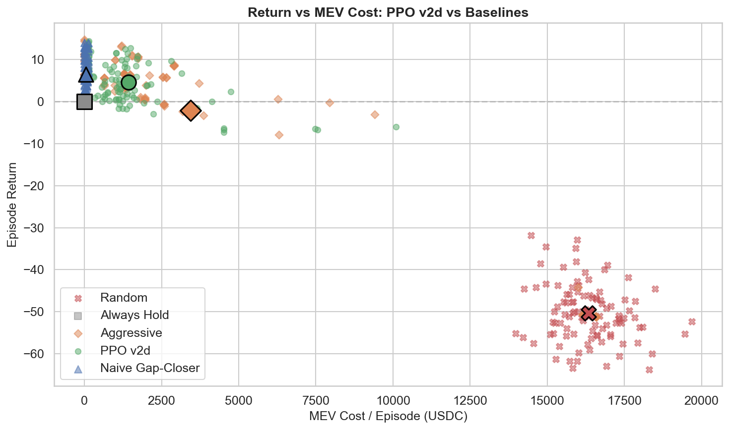
Baselines
- TWAP: The standard. Split $Q$ evenly over $T$ blocks.
- VWAP: Execute proportional to historical volume profiles.
- Adaptive: Hand-coded heuristics (urgency based on time/inventory).
Results
1. The Complexity Frontier
When does adaptivity actually pay off?
(Figure 2: Complexity Frontier — PPO-LSTM outperforms baselines primarily in high-contrast regime switching environments)
Let $\Delta$ denote the paper’s scalar performance score (higher is better), which aggregates execution quality (cost, risk, completion penalties) relative to TWAP. The frontier is a deployment rule: if your MEV environment is near-stationary, prefer heuristics; if it exhibits high-contrast latent switching, recurrent policies can pay.
- Low Contrast ($\kappa \approx 1\times$): TWAP wins. PPO-LSTM underperforms TWAP significantly ($\Delta_{RL} = -0.27$).
- Regime 100$\times$ (latent switching with high $\kappa$ contrast): PPO-LSTM wins. In the extreme regime-switching setting, PPO-LSTM significantly outperforms TWAP ($\Delta_{RL} = +2.88$).
- Correlated: Mixed. PPO-LSTM underperforms TWAP ($\Delta_{RL} = -0.53$), but Phase B results show that SAC can exploit correlation ($\Delta_{SAC} = +0.83$).
Evidence Ledger (don't skip):
- Where PPO-LSTM loses: Across the main benchmark, recurrent PPO is competitive but not uniformly superior — TWAP/Adaptive beat PPO-LSTM in stationary, state-dependent, fatigue, and time-varying settings (see Table 10 in the paper).
- Where PPO-LSTM wins: PPO-LSTM’s clear win appears in the extreme regime-switching (100$\times$ $\kappa$-contrast) setting ($\Delta = +2.88$), while moderate regimes are often non-significant.
- Why you still care: Optimizer choice can reverse outcomes (SAC flips Correlated); and OOD stress tests show raw PPO-LSTM has large boundary failures, motivating hybrid guardrails.
Conclusion: RL can win when the environment has exploitable non-stationary structure — but strong heuristics remain hard baselines, and robustness is the real bottleneck. These results describe within-model equilibrium pressure; real-world MEV is richer.
2. Algorithm Sensitivity ("Phase B")
We tested different RL algorithms. Result: Optimizer choice is first-order.
- In the Correlated regime, SAC (Soft Actor-Critic) significantly beat PPO-LSTM and TWAP. In Phase B, we gate SAC checkpoints at 4.0M and 5.0M steps, and both pass.
- In the Extreme regime, SAC (~-6.39) and TD3 (~-14.90) failed (underperformed TWAP), consistent with known sensitivity of off-policy methods under high variance / non-stationary targets.
So ‘better algorithm’ is regime-dependent: correlation helps SAC, extreme switching breaks it.
3. MEV Feedback
In ablations, adding realized MEV losses as feedback ($r_t \leftarrow r_t - \eta \cdot \text{MEV}_t$) improves adaptation by directly tagging attack-caused losses. We estimate MEV$_t$ as the sandwich-induced price degradation relative to the no-attack counterfactual (same action in the same AMM state, but without the attacker transactions). This isolates attack-induced slippage from ordinary impact and closes the credit assignment loop: without it, the agent often attributes poor fills to its own pacing rather than to being sandwiched.
4. Adaptation Speed: Detecting Regimes in 4 Steps
We measured how quickly the recurrent policy adapts after regime changes. Empirically, the policy’s actions are most sensitive to Inventory ($q_{rem}$), Volume ($V_t$), and Spread ($s_t$). Quantitatively, after a regime change the LSTM policy reaches ~90% of the optimal action adjustment within 4 steps.
5. Mechanism: Attack Rate Reduction
In regime-switching, PPO-LSTM cuts the attack rate from 38.2% (TWAP) to 14.3% and reduces MEV costs disproportionately; most of the total-cost gain comes from MEV evasion (69%), not just lower IS (47%).
(Figure 3: Policy Execution Mechanics — The agent learns to pause during high-MEV spikes (red zones) and execute aggressively when the coast is clear)
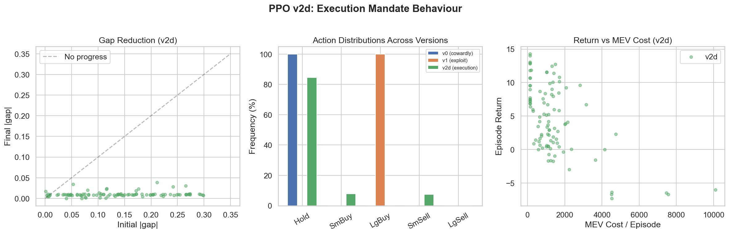
Action distributions become multimodal: aggressive modes in low-MEV, conservative modes in high-MEV, which specifically confounds searcher targeting. In plain English: the policy ‘probes’ and ‘pounces’—small noisy trades to avoid being an easy target, then larger trades when it infers a safer window. (Not a hard-coded heuristic — this emerges from the learned action distribution. This behavior is most visible in regime-switching environments.)
Discussion
The "Safety Shield"
In Out-Of-Distribution (OOD) tests, raw PPO-LSTM agents sometimes failed catastrophically:
- Liquidity Desert: $\Delta = -7.29$ (PPO-LSTM - TWAP)
- Tight Deadline: $\Delta = -14.38$ (PPO-LSTM - TWAP)
We introduced a deterministic Safety Shield: a minimum participation-rate constraint. If remaining inventory / remaining time exceeds a threshold, we force a minimum trade size per step. This recovered performance to near-TWAP levels in worst-case scenarios (e.g., Tight Deadline $\Delta = +0.12$). This is a hybrid-policy robustness benefit, not pure-policy robustness. Hybrid policies (RL + Guardrails) are the path to production.
Systemic Risk
If every trader uses these algorithms, they might synchronize from shared signals (e.g., shared MEV regime inference)—all withdrawing liquidity during high-MEV regimes and rushing back in during low-MEV regimes. If many agents learn similar regime detectors, they may synchronize even without communication. This could create liquidity black holes and flash crashes. The systemic equilibrium of many AI agents is an open research question.
Citation
If you use this work, please cite the working paper:
@unpublished{kemper2026equilibrium,
  title  = {Equilibrium Execution: Game-Theoretic Optimal Trading Under Endogenous MEV on Automated Market Makers},
  author = {Kemper, Lucas},
  note   = {Working paper},
  year   = {2026}
}