Introduction
This post summarizes my paper Equilibrium Execution: A Stackelberg Model of AMM Trading Under Endogenous MEV.
The question is: what does optimal execution look like on a public AMM when other agents can watch the trade, infer intent, and react?
Classical execution models usually treat market impact as an external cost. A large trader decides how quickly to trade, balancing immediate price impact against the risk of waiting. That framing is useful, but it misses something important on public decentralized exchanges. On an AMM, pool reserves are visible, transaction intent can leak through the mempool, and searchers can front-run, back-run, or sandwich predictable flow.
So the cost of execution is not only about trade size. It also depends on how the trader behaves and how searchers respond.
The paper calls this endogenous MEV. A trading schedule is also a signal. A deterministic TWAP can be efficient under a simple impact model, but it can also become easy to attack. A noisy or adaptive policy can hide intent better, but it may pay more timing risk or fail to complete under stress.
The main result is deliberately cautious: PPO-LSTM is competitive in some settings, but it does not uniformly beat strong static or heuristic baselines. The more useful contribution is the framework: model execution as a strategic game, calibrate adversaries from on-chain sandwich data, test algorithm sensitivity, and add deterministic safety guards before treating any learned policy as deployment-ready.
Execution as a Stackelberg Game
The paper models the trader-searcher interaction as a Stackelberg game.
The leader is a large trader choosing an execution policy $\pi_T$, which splits a target order $Q$ over a horizon of $T$ blocks. The followers are MEV searchers. They observe the trader’s behavior, or signals of it, and choose whether and how to extract value.
The trader minimizes total cost:
$$ J_T(\pi_T) = \mathbb{E}\left[\mathrm{IS} + \sum_{t=1}^T M_t(\pi_T, \pi_S)\right], $$
where $\mathrm{IS}$ is implementation shortfall and $M_t$ is MEV extracted at step $t$.
But the important part is that the searcher is not fixed. At equilibrium, the searcher best-responds to the trader:
$$ \pi_S = \mathrm{BR}(\pi_T). $$
So the trader is really minimizing:
$$ J_T(\pi_T) = \mathbb{E}\left[\mathrm{IS} + \sum_{t=1}^T M_t(\pi_T, \mathrm{BR}(\pi_T))\right]. $$
That is the core modeling move. MEV is not added afterward as a surcharge. It is generated by the interaction between the execution policy and the adversary’s response.
AMM Mechanics and Sandwich Extraction
The venue is a constant-product AMM in the Uniswap v2 style. The pool has reserves $(R_X, R_Y)$ and invariant:
$$ R_X R_Y = L^2. $$
Ignoring fees for exposition, swapping $\Delta x$ units of asset $X$ returns:
$$ \Delta y = R_Y - \frac{L^2}{R_X + \Delta x} = \frac{R_Y \Delta x}{R_X + \Delta x}. $$
The average execution price is:
$$ p_{\mathrm{exec}}(\Delta x) = \frac{\Delta y}{\Delta x} = \frac{R_Y}{R_X + \Delta x}. $$
This price worsens with trade size. Splitting an order reduces instantaneous impact, but it also creates more observable opportunities for searchers.
A sandwich attack has three legs:
- the searcher trades before the victim to move the AMM price;
- the victim executes at the worse price;
- the searcher trades back to unwind and capture the spread.
In the stylized CPAMM model used in the paper, the optimal front-run size against a victim trade $q$ is approximately:
$$ q^{F*} = \frac{R_X}{2}\left(\sqrt{1 + \frac{4q}{R_X}} - 1\right) - \frac{q}{2} + O(c_{\mathrm{gas}}). $$
For small trades $q \ll R_X$, the attack size is roughly proportional to the victim trade size. That is why predictability matters. If a searcher can infer the trader’s next slice, it can size the attack more accurately. If the trader introduces controlled variance, that sizing problem becomes noisier.
The theory section also gives a stylized result: under non-zero MEV intensity, deterministic TWAP is generically exploitable. That does not mean RL beats TWAP everywhere. It means that once MEV responds to the trader’s policy, deterministic schedules are not automatically safe.
Five MEV Regimes
The experiments test five adversary regimes. Each one changes the searcher intensity parameter $\kappa$, which controls how aggressively profitable opportunities are attacked.
| Regime | Searcher behavior | Why it matters |
|---|---|---|
| Stationary | Constant $\kappa$ | Lowest-complexity case; simple schedules are hard to beat. |
| State-dependent | $\kappa$ varies with observable state, such as volume or volatility | Tests whether the policy can react to market signals. |
| Regime-switching | Latent HMM state controls $\kappa$ | Tests memory and belief-state tracking. |
| Fatigue | Searcher intensity drops after repeated attacks | Models capital limits or cooldown behavior. |
| Time-varying | Sinusoidal intensity pattern | Captures deterministic activity cycles. |
The regime-switching setting is the most natural place to expect recurrent policies to help, because the true MEV state is not directly observed. The policy has to infer it from histories of prices, reserves, volume, spread, gas, inventory, and realized costs.
Learning Setup
The trader’s problem is cast as an episodic MDP. Each episode is a fresh execution task: trade a target quantity $Q$ over $T$ blocks while minimizing implementation shortfall, MEV losses, and failure-to-complete penalties.
The policy observes market and execution features:
| Feature | Meaning |
|---|---|
| $p_t$ | Current AMM mid-price |
| $R_X^t, R_Y^t$ | Pool reserves |
| $\sigma_t$ | Rolling volatility |
| $V_t$ | Recent trading volume |
| $q_{\mathrm{rem}}$ | Remaining inventory |
| $\tau_t$ | Normalized time |
| $\mathrm{IS}_t$ | Implementation shortfall so far |
| $s_t$ | Effective spread |
| $g_t$ | Gas price / MEV proxy |
The main learned policy is PPO with LSTM memory. The LSTM is included because the adversary state can be latent. A feed-forward MLP baseline is also trained, because recurrence should earn its keep rather than be assumed useful.
The reward penalizes execution cost, MEV, and failure to complete:
$$ r_t = -(p_{\mathrm{exec},t} - p_0)q_t - \alpha M_t - \beta \cdot \mathrm{completion\ penalty}. $$
The paper also tests MEV-feedback reward shaping:
$$ r_t^{\mathrm{MEV\text{-}fb}} = r_t - \eta M_t^{\mathrm{realized}}. $$
That term helps with credit assignment. Without realized MEV feedback, the policy only sees that some trajectory was expensive. With feedback, the policy gets a more direct signal that a specific action created extraction risk.
Iterated Best Response
Solving the exact Stackelberg problem with continuous neural policies is not practical. The paper uses Iterated Best Response (IBR) as an approximation.
The loop is:
- fix the trader policy and fit the searcher’s best response;
- fix the searcher and train the trader against that adversary;
- repeat until the trader policy and evaluation metrics stabilize.
The searcher is represented as a parameterized best-response function rather than as a full learned RL agent. Attack probability is smoothed by $\kappa$:
$$ P(\mathrm{attack}\mid q_t) = \kappa \cdot \sigma\left(\frac{\Pi_S(q_t, q_t^{F*}) - c_{\mathrm{threshold}}}{c_{\mathrm{scale}}}\right), $$
where $\Pi_S$ is expected sandwich profit. This gives the trader an adaptive adversary without requiring full co-evolution between two learned agents.
Calibration to On-Chain Sandwich Data
A key part of the paper is calibration. The adversary model is not purely synthetic. The paper estimates $\kappa$ from public Ethereum data using Google BigQuery and the Uniswap v2 WETH/USDC pool:
0xb4e16d0168e52d35cacd2c6185b44281ec28c9dc
The detector searches for within-block transaction triples matching the sandwich pattern: same attacker wallet on the front-run and back-run legs, a victim transaction in between, positive attacker profit, positive victim size, and bounded transaction-index proximity.
The calibration dataset is:
| Calibration field | Value |
|---|---|
| Raw detected sandwich rows | 3,427 |
| Clean rows used for HMM fit | 2,306 |
| Earliest timestamp | 2020-06-02 11:11:42 UTC |
| Latest timestamp | 2026-02-11 20:57:35 UTC |
| Low-intensity $\kappa_L$ | 0.001135 |
| High-intensity $\kappa_H$ | 0.979657 |
| $p_{LH}$ | 0.376230 |
| $p_{HL}$ | 0.343033 |
| Mean duration, low regime | 2.658 blocks |
| Mean duration, high regime | 2.915 blocks |
| Regime separation | 0.978522 |
The fitted adversary is a two-state Gaussian HMM. It produces a low-MEV and high-MEV regime with short but persistent durations. That calibrated process is then used for cross-evaluation against policies trained in stylized environments.
Main Benchmark: Strong Baselines Remain Hard
The most important empirical point is negative: PPO-LSTM does not dominate.
In the main benchmark, learned policies are competitive in several settings, but TWAP and adaptive heuristics remain difficult baselines.
| Regime | PPO-LSTM return | Strongest listed baseline | Reading |
|---|---|---|---|
| Stationary | $+3.20 \pm 0.02$ | TWAP: $+3.47 \pm 0.01$ | PPO loses to simple pacing. |
| Regime-switching | $+2.03 \pm 0.24$ | Adaptive: $+2.15 \pm 0.20$ | PPO is near TWAP but below Adaptive. |
| State-dependent | $+3.42 \pm 0.02$ | TWAP: $+3.83 \pm 0.01$ | Correlation alone is not enough for PPO. |
| Fatigue | $+4.22 \pm 0.02$ | Adaptive: $+4.40 \pm 0.00$ | Heuristics exploit the simpler structure. |
| Time-varying | $+3.10 \pm 0.01$ | Adaptive: $+3.27 \pm 0.01$ | Periodic structure does not require LSTM complexity. |
The clean reading is: there is no universal PPO win. Learned recurrent policies are not a plug-in replacement for TWAP, VWAP, or simple adaptive schedules. Added complexity is only worth it when the adversary structure is hard enough, learnable enough, and stable enough to survive robustness checks.
Complexity Frontier: Useful, but Not a Blanket Win
The complexity frontier asks when extra model expressiveness is worth the cost.
The answer is mixed. In one high-contrast single-run regime-switching setting, PPO looks strong. But the consolidated multi-seed validation is more conservative. The A3 extreme-regime result has wide uncertainty and includes a catastrophic seed:
$$ \Delta_{\mathrm{PPO}-\mathrm{TWAP}} = -15.10, \quad 95%\ \mathrm{CI} = [-43.25, +0.65], \quad p = 0.31. $$
So the right conclusion is not “LSTMs beat TWAP in hard regimes.” The better conclusion is: high-contrast latent structure can create opportunities for learned policies, but the advantage has to survive seed sensitivity, optimizer choice, and OOD stress.
The memory ablations also do not support a blanket recurrent-policy claim. In some tested stationary and regime settings, the MLP variant is stronger than the LSTM variant.
Algorithm Sensitivity: Optimizer Choice Is First-Order
The Phase B experiments compare SAC, TD3, and recurrent PPO under identical environments. The rankings change sharply by regime.
| Experiment | Algorithm | Environment | Return | $\Delta$ vs TWAP | Status |
|---|---|---|---|---|---|
| B1 | SAC | Extreme regime | $-9.53 \pm 21.60$ | $-6.39$ | Complete |
| B2 | TD3 | Extreme regime | $-18.04 \pm 26.11$ | $-14.90$ | Complete |
| B3 | SAC | Correlated | $+0.98 \pm 0.15$ | $+0.83$ | Complete |
| B4 | TD3 | Correlated | $-0.56 \pm 0.33$ | $-0.71$ | Complete |
| B5 | Recurrent PPO | Correlated | $-0.47 \pm 0.52$ | $-0.61$ | Complete |
The clearest positive result in this block is SAC in the correlated regime. Pre-registered SAC checkpoints at 4.0M and 5.0M steps both pass, with $\Delta_{\mathrm{SAC}-\mathrm{TWAP}} = +0.87$ and $+0.83$.
But in the extreme regime, both SAC and TD3 underperform TWAP. So optimizer choice is not a tuning footnote. It changes the empirical conclusion.
Calibrated vs. Stylized Transfer
The paper cross-evaluates policies trained under calibrated HMM dynamics and stylized dynamics. Matched-budget results show near parity on calibrated dynamics and a small stylized edge on stylized dynamics.
| Environment | Calibrated policy | Stylized policy | $\Delta$ (Stylized - Calibrated) |
|---|---|---|---|
| Calibrated environment | $+3.705$ | $+3.662$ | $-0.043$ |
| Stylized environment | $+3.274$ | $+3.323$ | $+0.049$ |
| As-run means | $+3.705$ | $+3.323$ | $-0.382$ |
The calibrated-environment gap is not statistically decisive ($\Delta_{S-C}=-0.04$, $p=0.35$). The stylized environment favors the stylized policy by a small but statistically significant amount ($\Delta_{S-C}=+0.05$, $p<0.001$).
The as-run aggregate favors calibrated training, but that aggregate mixes native-environment and transfer effects. I read this as asymmetric transfer evidence, not as proof that calibrated training is always better.
What the Policy Learns
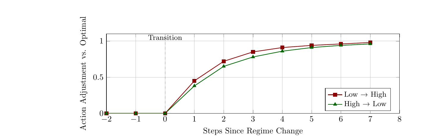
The learned behavior is easiest to interpret in regime-switching diagnostics. In those runs, the LSTM learns a regime-sensitive execution style:
| Inferred condition | Learned behavior |
|---|---|
| High-MEV regime | Reduces trade sizes, increases action variance, and delays large trades. |
| Low-MEV window | Increases trade sizes to catch up, reduces variance, and builds a completion buffer. |
| Near deadline | Becomes aggressive even when MEV risk is high, because completion starts to dominate. |
The transition diagnostics suggest that the policy adapts within a few steps after regime changes in the tested setting. I would treat those numbers as diagnostic rather than universal, but they are consistent with the idea that memory helps when the adversary state is latent.
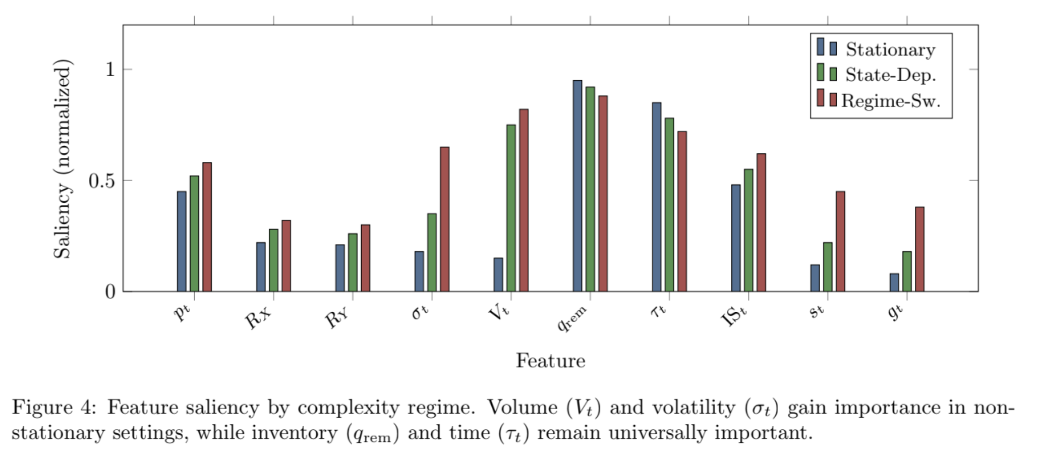
Feature-saliency analysis points in the same direction. Inventory and time dominate across regimes, while volume, spread, and gas become more important in non-stationary and regime-switching settings.
One appendix diagnostic slice is favorable to PPO-LSTM:
| Strategy | IS (%) | MEV (%) | Total cost (%) | Sharpe | Completion (%) | Attack rate (%) |
|---|---|---|---|---|---|---|
| TWAP | 0.53 | 0.45 | 0.98 | 0.91 | 100.0 | 38.2 |
| VWAP | 0.49 | 0.41 | 0.90 | 0.99 | 100.0 | 35.1 |
| PPO-MLP | 0.42 | 0.31 | 0.73 | 1.32 | 100.0 | 28.1 |
| PPO-LSTM | 0.28 | 0.14 | 0.42 | 2.38 | 100.0 | 14.3 |
| Oracle | 0.18 | 0.08 | 0.26 | 3.52 | 100.0 | 8.5 |
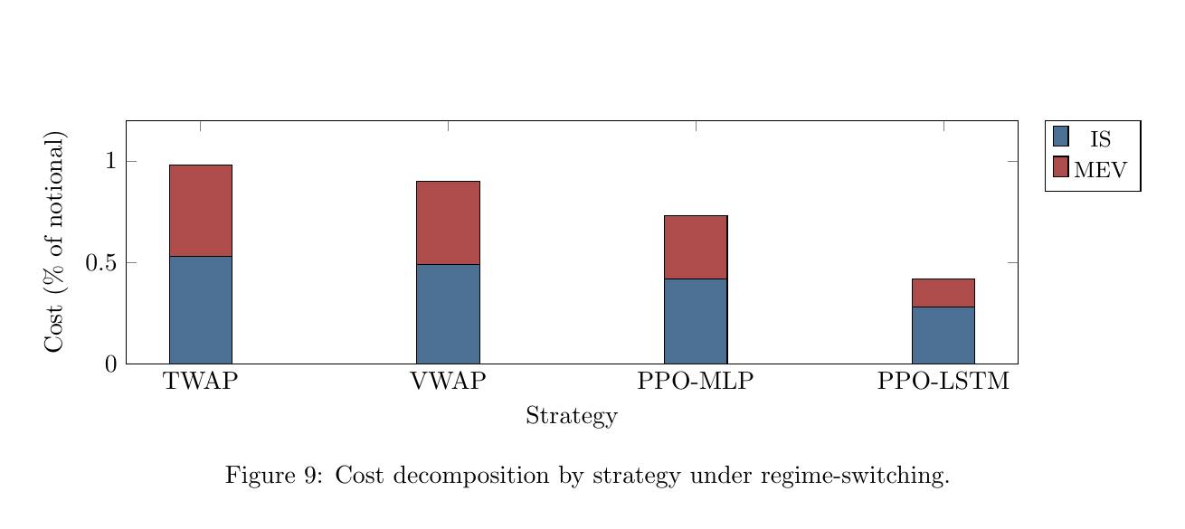
In that slice, PPO-LSTM cuts MEV much more than it cuts implementation shortfall. The useful behavior is not just smoother execution. It is MEV evasion.
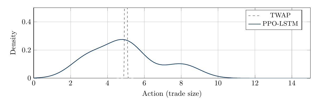
The action distribution also changes. TWAP is a spike. PPO-LSTM is multimodal: smaller trades in high-MEV states, larger trades in low-MEV windows, and intermediate behavior during transitions.
OOD Stress: Where Raw PPO Breaks
The out-of-distribution tests are the strongest argument for guardrails. Raw PPO underperforms TWAP across all pooled OOD scenarios, with the largest failures under tight deadlines and liquidity deserts.
| Scenario | Stressor | Raw PPO - TWAP | Fill, PPO/TWAP | Reading |
|---|---|---|---|---|
| Liquidity desert | Pool depth divided by 5 | $-7.29$ | 47.3% / 50.2% | Learned policy fails under severe liquidity collapse. |
| Tight deadline | Deadline halved to 25 blocks | $-14.38$ | 84.6% / 99.2% | PPO waits too long and cannot recover. |
| Jared attack | Monopolist searcher, $\kappa=1$ | $-0.26$ | 99.8% / 99.9% | Small but significant degradation. |
| Flash crash | Volatility $\times 3$ | $-0.25$ | 99.8% / 99.9% | Small but significant degradation. |
| Regime churn | Regime persistence collapse | $-0.18$ | 99.9% / 99.9% | Churn hurts, but does not break completion. |
The pooled OOD result is:
$$ \Delta_{\mathrm{PPO}-\mathrm{TWAP}} = -2.86, \quad 95%\ \mathrm{CI} = [-3.11, -2.61], \quad p < 0.001. $$
This is the deployment-relevant result. A learned policy can look reasonable in-distribution and still fail at the boundary.
The Safety Shield
To reduce boundary failures, the paper adds a deterministic safety shield. It enforces a minimum participation rate when remaining inventory divided by remaining time gets too high.
This is not pure RL robustness. It is a hybrid policy: learned execution plus deterministic override. But for real execution, that is probably the right shape.
| Scenario | Shielded PPO - TWAP | Shielded PPO - Raw PPO | Trigger rate |
|---|---|---|---|
| Jared attack | $+0.03$ | $+0.29$ | 47.9% |
| Flash crash | $+0.03$ | $+0.29$ | 47.7% |
| L2 migration | $+0.06$ | $+0.24$ | 47.6% |
| Liquidity desert | $+0.00$ | $+7.29$ | 100.0% |
| Tight deadline | $+0.12$ | $+14.50$ | 97.0% |
| Post-Dencun gas | $+0.07$ | $+0.19$ | 47.6% |
| Gas spike | $+0.06$ | $+0.27$ | 47.6% |
| Regime churn | $-0.03$ | $+0.16$ | 46.9% |
The shield recovers the worst failures to near-TWAP behavior without retraining. In the tight-deadline scenario, it raises PPO fill from 84.6% to 99.3%, essentially matching TWAP’s 99.2%.
The lesson is simple: a model that can choose to wait needs a hard rule for when waiting becomes dangerous.
Practical Takeaways
For traders, I would summarize the paper as four rules.
First, do not treat MEV as a fixed fee. Execution policies are signals, and signals invite strategic response.
Second, match policy complexity to the environment. Stationary, fatigue, and time-varying regimes may not need recurrent neural policies. Latent regimes might, but only if the advantage survives seeds, optimizers, and stress tests.
Third, include MEV-relevant signals in the feedback loop. Gas, spread, volume, and recent attack outcomes can matter, but their value is regime-dependent.
Fourth, do not deploy raw learned execution as an unconditional replacement for static schedules. The stronger design is hybrid: adaptive learned behavior inside deterministic completion and safety constraints.
For protocol designers, the results reinforce that trader-side adaptation and protocol-level mitigation interact. Private orderflow, batch auctions, and MEV redistribution mechanisms change the searcher’s best response, which changes the trader’s optimal policy.
Limitations
The paper is still a simulation study.
The environment is calibrated to public sandwich data, but it abstracts from cross-venue routing, private orderflow, heterogeneous searcher populations, strategic LP behavior, block inclusion uncertainty, and richer multi-block MEV strategies. The searcher is represented as a parameterized best response rather than as a full population of competing bots.
The calibration is also pool-specific: Uniswap v2 WETH/USDC. Other pools, AMM designs, chains, private relays, and liquidity regimes may produce different $\kappa$ dynamics.
Finally, the results are algorithm-sensitive. SAC, TD3, PPO, LSTM, and MLP variants can rank differently across environments. A serious deployment pipeline needs algorithm robustness checks, not just one trained checkpoint.
Conclusion
The core thesis is that DEX execution is strategic. A trader’s schedule changes what searchers believe, what they attack, and how much value they can extract. That makes MEV endogenous.
The evidence supports a cautious deployment thesis:
- model execution as a game, not as a single-agent control problem with a fixed MEV tax;
- calibrate adversary dynamics from on-chain data where possible;
- treat architecture and optimizer choice as empirical variables;
- report OOD failures instead of hiding them;
- pair learned policies with deterministic safety shields.
RL can discover useful evasive behavior, especially when adversary behavior is latent and non-stationary. But strong heuristics remain hard baselines, and robustness is the bottleneck.
So the best question is not “Does RL beat TWAP?” The better question is: under which adversary dynamics, with which optimizer, under which stress boundary, and with what guardrails?